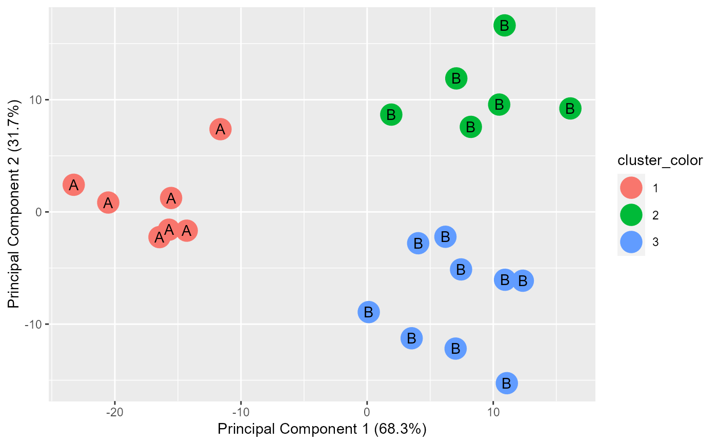
Make a 2D scatter plot that shows the data as represented by PC1 and PC2
generate.2D.clustering.with.labeled.subgroup.RdAfter clustering of a dataset with two or more dimensions, we often want to visualize the result of the clustering on a 2D plot. If there are more than two dimensions, we want to first reduce the data down to two dimensions. This can be done with PCA. After PCA is completed, the data can be plotted with this function.
generate.2D.clustering.with.labeled.subgroup(
  pca.results.input,
  cluster.labels.input,
  subgroup.labels.input
)
Arguments
| pca.results.input | An object outputted by stats::prcomp(). The PCA of all the features used for clustering. There should be at least 3 features. |
|---|---|
| cluster.labels.input | A vector of integers that specify which cluster each observation belongs to (order of observations must match the data inputted to prcomp() to generate pca.results.input). |
| subgroup.labels.input | A vector of strings that specify an additional label for each observations. |
Value
A list of 4 objects: 1.ggplot objct for PC1 vs PC2. 2.ggplot object for PC1 vs PC3. 3.Chi-square results. 4.Table used for chi-square.
Details
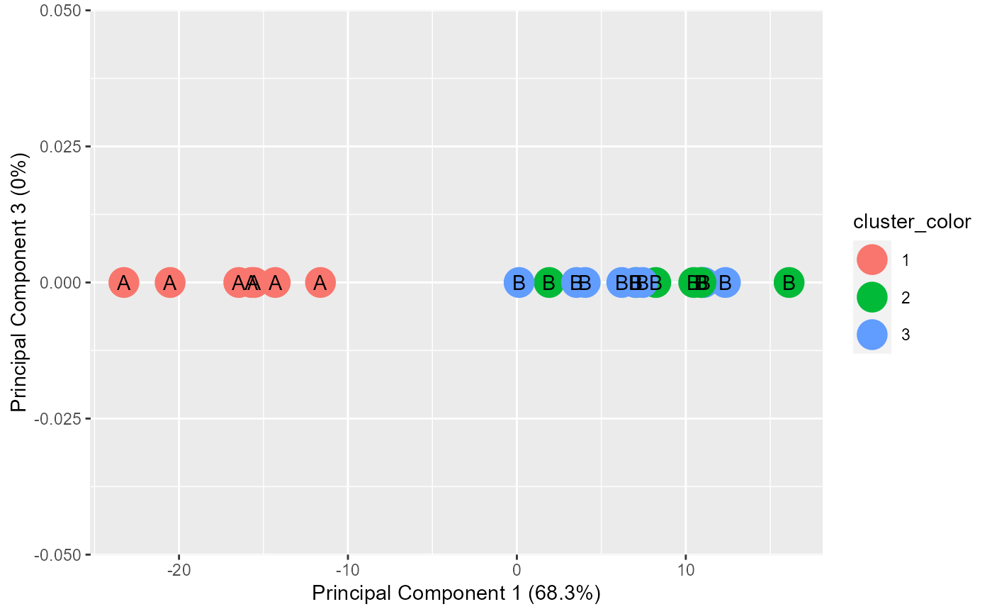
This function plots PC1 vs PC2 as well as PC1 vs PC3. This function uses the output of stat::prcomp(). The input into prcomp() needs to have at least 3 dimensions. Points are colored by the cluster input and they are labeled by the subgroup input.
Additionally, this function also calculates chi-square results to see if cluster.labels.input and subgroup.labels.input are associated.
See also
Other Clustering functions:
CalcOptimalNumClustersForKMeans(),
GenerateParcoordForClusters(),
HierarchicalClustering(),
generate.3D.clustering.with.labeled.subgroup(),
generate.plots.comparing.clusters()
Examples
example.data <- data.frame(x = c(18, 21, 22, 24, 26, 26, 27, 30, 31, 35, 39, 40, 41, 42, 44, 46, 47, 48, 49, 54, 35, 30), y = c(10, 11, 22, 15, 12, 13, 14, 33, 39, 37, 44, 27, 29, 20, 28, 21, 30, 31, 23, 24, 40, 45), z = c(1, 1, 1, 1, 1, 1, 1, 1, 1, 1, 1, 1, 1, 1, 1, 1, 1, 1, 1, 1, 1, 1)) #dev.new() plot(example.data$x, example.data$y)km.res <- stats::kmeans(example.data[,c("x", "y", "z")], 3, nstart = 25, iter.max=10) grouped <- km.res$cluster pca.results <- prcomp(example.data[,c("x", "y", "z")], scale=FALSE) actual.group.label <- c("A", "A", "A", "A", "A", "A", "A", "B", "B", "B", "B", "B", "B", "B", "B", "B", "B", "B", "B", "B", "B", "B") results <- generate.2D.clustering.with.labeled.subgroup(pca.results, grouped, actual.group.label)#> Warning: Chi-squared approximation may be incorrect#PC1 vs PC2 results[[1]]#PC1 vs PC3 results[[2]]#Chi-square results results[[3]]#> #> Pearson's Chi-squared test #> #> data: tbl #> X-squared = 22, df = 2, p-value = 1.67e-05 #>#Table results[[4]]#> cluster.labels.input #> subgroup.labels.input 1 2 3 #> A 7 0 0 #> B 0 6 9