Generate plots to help decide optimal number of clusters for Kmeans
CalcOptimalNumClustersForKMeans.RdMultiple methods are included for assessing optimal number of clusters.
CalcOptimalNumClustersForKMeans(inputted.data, clustering.columns)
Arguments
| inputted.data | A dataframe. |
|---|---|
| clustering.columns | Name of columns with data to use for kmeans clustering. |
Value
A list is returned with two elements:
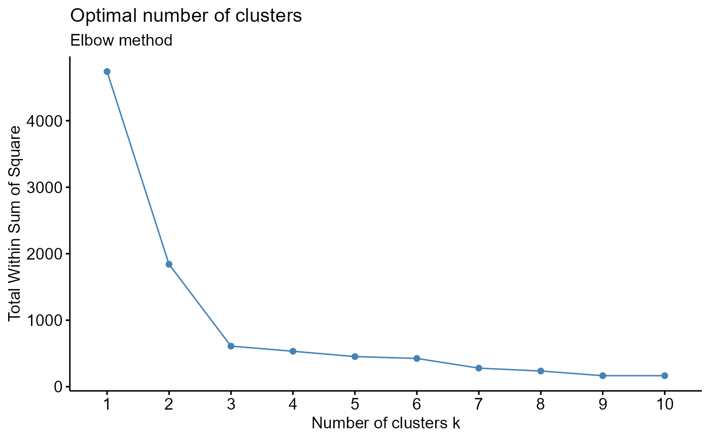
ggplot for elbow plot.
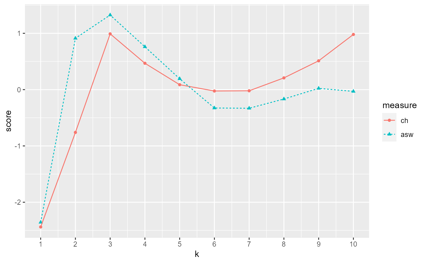
ggplot for ch and asw plot.
Details
Function generates plots that allow you to evaluate optimal number of clusters using 3 different methods:
Elbow method: https://www.datanovia.com/en/lessons/determining-the-optimal-number-of-clusters-3-must-know-methods/. Plot intra-cluster variation. Pick the K (cluster) corresponding to a sharp decrease (the elbow).
Calinski-Harabasz Index (ch) method: https://www.datasciencecentral.com/profiles/blogs/machine-learning-unsupervised-k-means-clustering-and and https://medium.com/@haataa/how-to-measure-clustering-performances-when-there-are-no-ground-truth-db027e9a871c
Average Silhouette Width (asw) method: https://www.datasciencecentral.com/profiles/blogs/machine-learning-unsupervised-k-means-clustering-and and https://medium.com/@haataa/how-to-measure-clustering-performances-when-there-are-no-ground-truth-db027e9a871c
ch and asw both produce a score. Higher score = better defined cluster. Maximize between cluster dispersion and minimize within cluster dispersion. Can plot the score versus the number of clusters.
See also
Other Clustering functions:
GenerateParcoordForClusters(),
HierarchicalClustering(),
generate.2D.clustering.with.labeled.subgroup(),
generate.3D.clustering.with.labeled.subgroup(),
generate.plots.comparing.clusters()
Examples
example.data <- data.frame(x = c(18, 21, 22, 24, 26, 26, 27, 30, 31, 35, 39, 40, 41, 42, 44, 46, 47, 48, 49, 54, 35, 30), y = c(10, 11, 22, 15, 12, 13, 14, 33, 39, 37, 44, 27, 29, 20, 28, 21, 30, 31, 23, 24, 40, 45)) #dev.new() plot(example.data$x, example.data$y)#Results should say that 3 clusters is optimal output <- CalcOptimalNumClustersForKMeans(example.data, c("x", "y")) elbow.plot <- output[[1]] ch.and.asw.plot <- output[[2]] #dev.new() elbow.plot#dev.new() ch.and.asw.plot