Automated plotting of time series, PSD, and log transformed PSD
AutomatedCompositePlotting.RdThis function uses a lot of the functions in this package (psdr) to automate the plotting process for plotting composite curves and having multiple curves on the same plot.
AutomatedCompositePlotting(
  list.of.windows,
  name.of.col.containing.time.series,
  x_start = 0,
  x_end,
  x_increment,
  level1.column.name,
  level2.column.name,
  level.combinations,
  level.combinations.labels,
  plot.title,
  plot.xlab,
  plot.ylab,
  combination.index.for.envelope = NULL,
  TimeSeries.PSD.LogPSD = "TimeSeries",
  sampling_frequency = NULL,
  my.colors = c("blue", "red", "black", "green", "gold", "darkorchid1", "brown",
    "deeppink", "gray")
)
Arguments
| list.of.windows | A list of windows (dataframes). All windows should have the same length, but because interpolation is used, the function still works if window length differs. |
|---|---|
| name.of.col.containing.time.series | A string that specifies the name of the column in the windows that correspond to the time series that should be used. |
| x_start | Numeric value specifying start of the new x-axis. Default is 0. |
| x_end | Numeric value specifying end of the new x-axis. For PSD, maximum value is the sampling_frequency divided by 2. |
| x_increment | Numeric value specifying increment of the new x-axis. |
| level1.column.name | A String that specifies the column name to use for the first level. This column should only contain one unique value within each window. |
| level2.column.name | A String that specifies the column name to use for the second level. This column should only contain one unique value within each window. |
| level.combinations | A List containing Lists. Each list that it contains has two vectors. The first vector specifying the values for level1 and the second vector specifying the values for level2. Each list element will correspond to a new line on the plot. |
| level.combinations.labels | A vector of strings that labels each combination. This is used for making the figure legend. |
| plot.title | String for title of plot. |
| plot.xlab | String for x-axis of plot. |
| plot.ylab | String for y-axis of plot. |
| combination.index.for.envelope | A numeric value that specifies which combination (index of level.combinations) should have a line with an error envelope. The default is no envelope. |
| TimeSeries.PSD.LogPSD | A String with 3 possible values to specify what type of plot to create from the time series: 1. "TimeSeries", 2. "PSD", 3. "LogPSD" |
| sampling_frequency | Numeric value used for specifying sampling frequency if PSD or LogPSD is made with this function. Default is NULL because default plot created is a time series plot. |
| my.colors | A vector of strings that specify the color for each line. 9 default values are used. |
Value
A List with three objects:
A List of dataframes containing values for each line on the plot. The order of the dataframes correspond to the order of the combinations in level.combinations.
A ggplot object that can be plotted right away.
If plot selected is a PSD, then a List is outputted from SingleBinPSDIntegrationOrDominantFreqComparison() to compare dominant frequencies between combinations.
Details
Given a list of windows, you can specify which windows you want to average together to form a curve on the plot. You can specify multiple combos and therefore multiple curves can be plotted on the same plot with a legend to specify the combo used to create each curve. An error envelope can also be created for a single curve on the plot.
The function automatically generates a ggplot for easy plotting. However, the function also outputs dataframes for each combo. Each dataframe has 3 columns:
X value: For timeseries, this will be in the original units that separates each observation in the time series. For example, if there are 150 observations and each observation is 0.02 seconds apart, then if 150 observations are specified as the x_increment, then each observation are still 0.02 seconds. The time difference between the first and last observation needs to equal the time difference between the first and last observation in the original time series. For PSD and LogPSd, the units will be in Hz (frequency). The frequency range depends on the sampling frequency. Smallest frequency is 0 and largest frequency is sampling_frequency/2.
Y value: For time series, this will be in the original units of the time series. For PSD, the units will be (original units)^2/Hz, for LogPSD, the units will be log((original units)^2/Hz)).
Standard deviation of Y value. This can be used to plot error bars or error envelopes to see the spread of the windows used to make the composite.
Three different plots can be created:
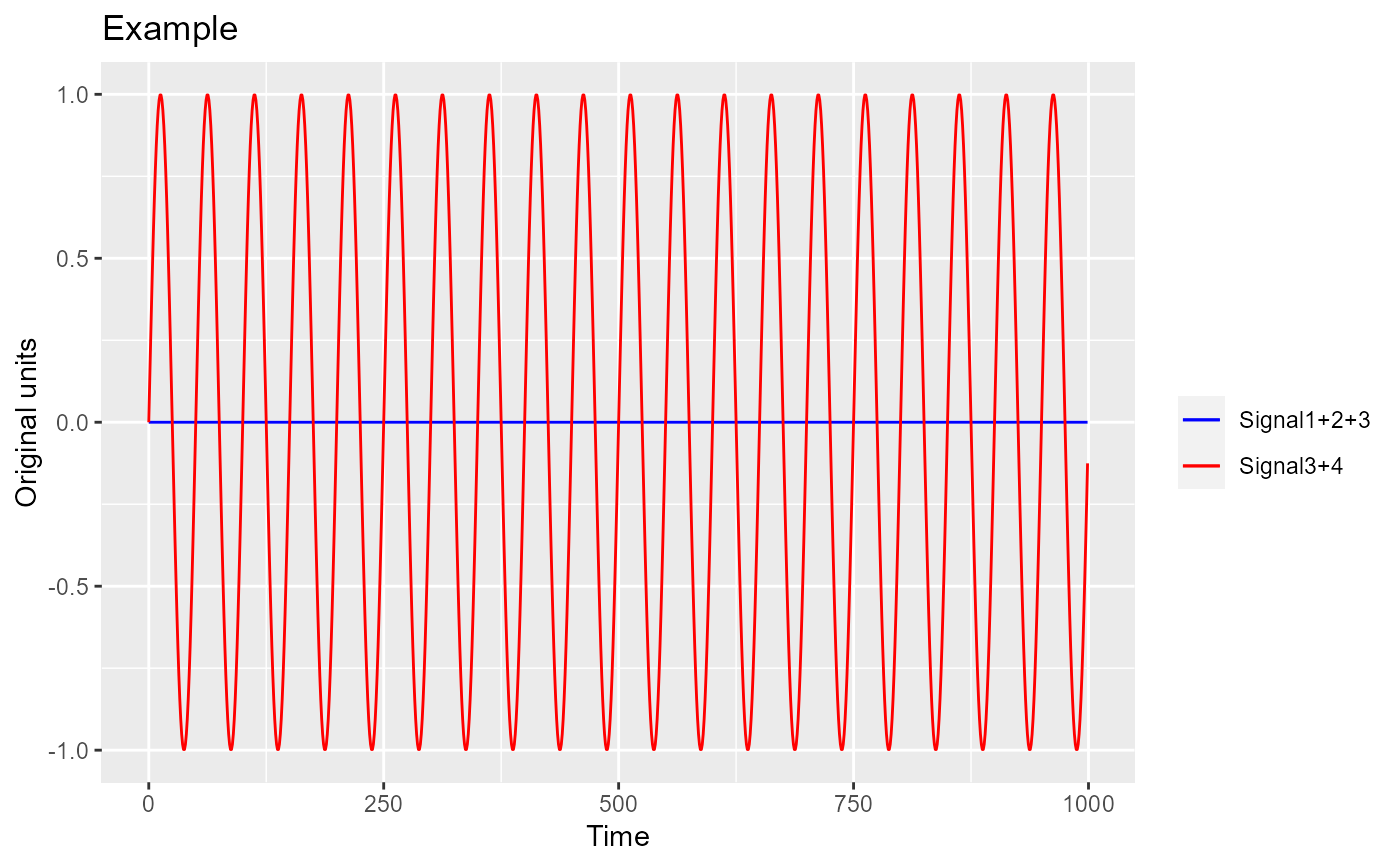
Time series plot. This simply takes the time series in the windows, averages them for each combo, and then plots the composite curve for each combo.
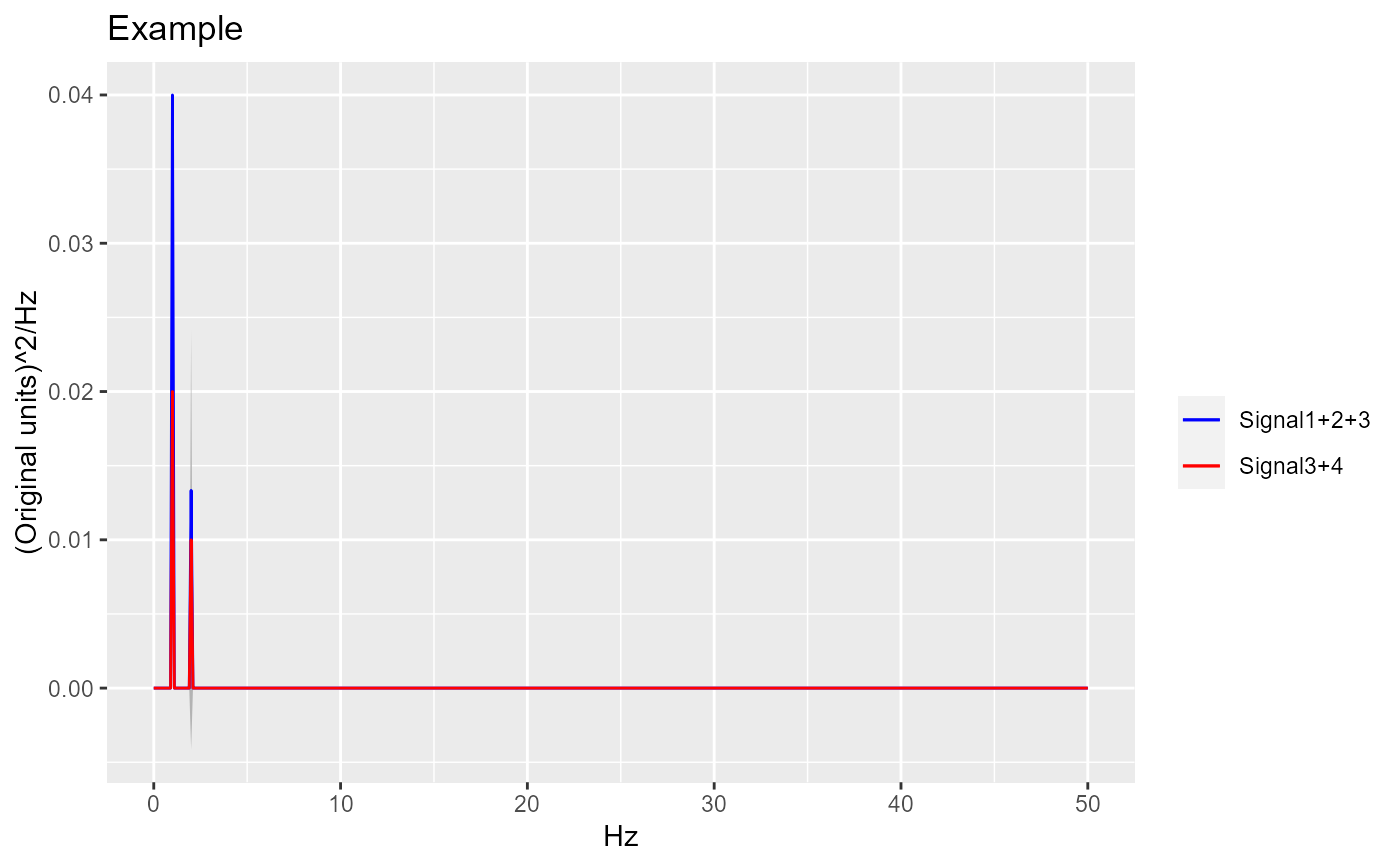
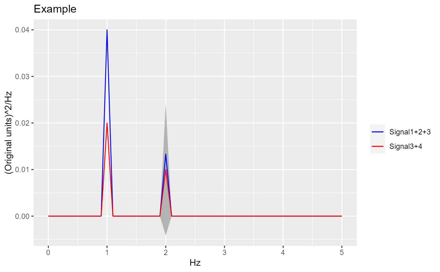
PSD plot. This takes the time series in the windows and given the sampling frequency, it calculates the PSD. It averages the PSD for the windows in each combo, and then plots the composite curve for each combo.
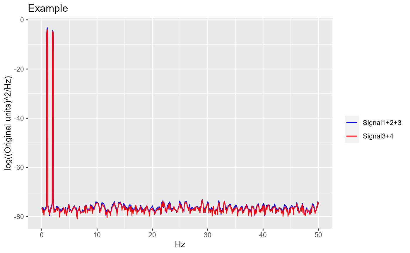
Log transformed PSD plot. Same as PSD plot except at the end, the composite PSD curves are log transformed.
Examples
#I want to create a plot that shows two curves: #1. Composite of time series signals 1, 2, and 3. #2. Composite of time series signals 3 and 4. #Create a vector of time that represent times where data are sampled. Fs = 100; #sampling frequency in Hz T = 1/Fs; #sampling period L = 1000; #length of time vector t = (0:(L-1))*T; #time vector #First signal #1. 1 Hz with amplitude of 2 S1 <- 2*sin(2*pi*1*t) level1.vals <- rep("a", length(S1)) level2.vals <- rep("1", length(S1)) S1.data.frame <- as.data.frame(cbind(t, S1, level1.vals, level2.vals)) colnames(S1.data.frame) <- c("Time", "Signal", "level1.ID", "level2.ID") S1.data.frame[,"Signal"] <- as.numeric(S1.data.frame[,"Signal"]) #Second signal #1. 1 Hz with amplitude of -4 #2. 2 Hz with amplitude of -2 S2 <- (-4)*sin(2*pi*1*t) - 2*sin(2*pi*2*t); level1.vals <- rep("a", length(S2)) level2.vals <- rep("2", length(S2)) S2.data.frame <- as.data.frame(cbind(t, S2, level1.vals, level2.vals)) colnames(S2.data.frame) <- c("Time", "Signal", "level1.ID", "level2.ID") S2.data.frame[,"Signal"] <- as.numeric(S2.data.frame[,"Signal"]) #Third signal #1. 1 Hz with amplitude of 2 #2. 2 Hz with amplitude of 2 S3 <- 2*sin(2*pi*1*t) + 2*sin(2*pi*2*t); level1.vals <- rep("a", length(S3)) level2.vals <- rep("3", length(S3)) S3.data.frame <- as.data.frame(cbind(t, S3, level1.vals, level2.vals)) colnames(S3.data.frame) <- c("Time", "Signal", "level1.ID", "level2.ID") S3.data.frame[,"Signal"] <- as.numeric(S3.data.frame[,"Signal"]) #Fourth signal #1. 1 Hz with amplitude of -2 S4 <- -2*sin(2*pi*1*t) level1.vals <- rep("b", length(S4)) level2.vals <- rep("3", length(S4)) S4.data.frame <- as.data.frame(cbind(t, S4, level1.vals, level2.vals)) colnames(S4.data.frame) <- c("Time", "Signal", "level1.ID", "level2.ID") S4.data.frame[,"Signal"] <- as.numeric(S4.data.frame[,"Signal"]) windows <- list(S1.data.frame, S2.data.frame, S3.data.frame, S4.data.frame) #Gets the composite of the first, second, and third signal. Should result in a flat signal. FirstComboToUse <- list( c("a"), c(1, 2, 3) ) #Gets the composite of the third and fourth signal SecondComboToUse <- list( c("a", "b"), c(3) ) #Timeseries----------------------------------------------------------------- timeseries.results <- AutomatedCompositePlotting(list.of.windows = windows, name.of.col.containing.time.series = "Signal", x_start = 0, x_end = 999, x_increment = 1, level1.column.name = "level1.ID", level2.column.name = "level2.ID", level.combinations = list(FirstComboToUse, SecondComboToUse), level.combinations.labels = c("Signal 1 + 2 + 3", "Signal 3 + 4"), plot.title = "Example", plot.xlab = "Time", plot.ylab = "Original units", combination.index.for.envelope = NULL, TimeSeries.PSD.LogPSD = "TimeSeries", sampling_frequency = NULL) ggplot.obj.timeseries <- timeseries.results[[2]] #Plot. Will see the 1+2+3 curve as a flat line. The 3+4 curve will only have 2 Hz. ##dev.new() ggplot.obj.timeseries#PSD------------------------------------------------------------------------- #Note that the PSDs are not generated directly from the "Signal 1 + 2 + 3" and #the "Signal 3 + 4" time series. Instead, PSDs are generated individually #for signals 1, 2, 3, and 4, and then then are summed together. PSD.results <- AutomatedCompositePlotting(list.of.windows = windows, name.of.col.containing.time.series = "Signal", x_start = 0, x_end = 50, x_increment = 0.01, level1.column.name = "level1.ID", level2.column.name = "level2.ID", level.combinations = list(FirstComboToUse, SecondComboToUse), level.combinations.labels = c("Signal 1 + 2 + 3", "Signal 3 + 4"), plot.title = "Example", plot.xlab = "Hz", plot.ylab = "(Original units)^2/Hz", combination.index.for.envelope = 2, TimeSeries.PSD.LogPSD = "PSD", sampling_frequency = 100)#> Warning: cannot compute exact p-value with tiesggplot.obj.PSD <- PSD.results[[2]] #Plot. For both plots, two peaks will be present, 1 Hz and 2 Hz. 1 Hz should be #stronger in both cases because more signals have this frequency (even if amp is negative). #Error envelope is specified for the second (red) curve. Envelope should only #be present for 2 Hz signal. #dev.new() ggplot.obj.PSD#PSD Zoomed in--------------------------------------------------------------- PSD.results <- AutomatedCompositePlotting(list.of.windows = windows, name.of.col.containing.time.series = "Signal", x_start = 0, x_end = 5, x_increment = 0.01, level1.column.name = "level1.ID", level2.column.name = "level2.ID", level.combinations = list(FirstComboToUse, SecondComboToUse), level.combinations.labels = c("Signal 1 + 2 + 3", "Signal 3 + 4"), plot.title = "Example", plot.xlab = "Hz", plot.ylab = "(Original units)^2/Hz", combination.index.for.envelope = 2, TimeSeries.PSD.LogPSD = "PSD", sampling_frequency = 100)#> Warning: cannot compute exact p-value with tiesggplot.obj.PSD <- PSD.results[[2]] #Plot. For both plots, two peaks will be present, 1 Hz and 2 Hz. 1 Hz should be #stronger in both cases because more signals have this frequency (even if amp is negative). #Error envelope is specified for the second (red) curve. Envelope should only #be present for 1 Hz signal. #dev.new() ggplot.obj.PSD#LogPSD------------------------------------------------------------------------- LogPSD.results <- AutomatedCompositePlotting(list.of.windows = windows, name.of.col.containing.time.series = "Signal", x_start = 0, x_end = 50, x_increment = 0.01, level1.column.name = "level1.ID", level2.column.name = "level2.ID", level.combinations = list(FirstComboToUse, SecondComboToUse), level.combinations.labels = c("Signal 1 + 2 + 3", "Signal 3 + 4"), plot.title = "Example", plot.xlab = "Hz", plot.ylab = "log((Original units)^2/Hz)", combination.index.for.envelope = NULL, TimeSeries.PSD.LogPSD = "LogPSD", sampling_frequency = 100) ggplot.obj.LogPSD <- LogPSD.results[[2]] #Plot. For both plots, two peaks will be present, 1 Hz and 2 Hz. 1 Hz should #be stronger in both cases because more signals have this frequency (even if amp is negative). #Error envelope is specified for the second (red) curve. Envelope should only #be present for 2 Hz signal. #dev.new() ggplot.obj.LogPSD