Generate a random forest model for different subsets of the data and display results into a matrix

RandomForestAutomaticMtryAndNtree() or randomForest() is used on each subset of the data. For each subset of the data: A random forest model is generated. This random forest model is used to make a single column in the final matrix which can be used to generate a pheatmap.

RandomForestClassificationGiniMatrixForPheatmap(
  input.data,
  factor.name.for.subsetting,
  name.of.predictors.to.use,
  target.column.name,
  seed,
  should.mtry.and.ntree.be.optimized = FALSE
)

Arguments

input.data	A dataframe.
factor.name.for.subsetting	String to specify name of column to use for subsetting. The column should be a factor. Each column of the generated pheatmap will correspond to a level in the factor.
name.of.predictors.to.use	A vector of strings to specify name of columns to use as predictors for random forest model. Each column should be numeric.
target.column.name	A string to specify the column with values the random forest model is trying to predict for. The column should be a factor.
seed	A number to set for random number generation.
should.mtry.and.ntree.be.optimized	A boolean to indicate if RandomForestAutomaticMtryAndNtree() should be used to optimize ntree and mtry. Default is FALSE.

Value

A list with three objects:

A numerical matrix that can be used for pheatmap generation.
A list of subset data sets for each column in the heatmap matrix.
A list of vectors containing the predictions for each column in the heatmap matrix. These values are used to calculate the MCC.
A list of RF objects, each object corresponding to one column in the heatmap matrix.

Details

In each column of the final matrix, the Matthew's Correlation Coefficient (MCC) is calculated and displayed as a row titled MCC.val to specify the performance of the model to predict the target in that particular data subset. Each column of the final matrix also has others rows, with each row specifying a single predictor used. For each predictor, the mean decrease in gini index is indicated in the matrix and can be used to determine how important the predictor is for predicting the target in that particular data subset.

The result from this function should be used with the RandomForestClassificationPercentileMatrixForPheatmap() function to create a pheatmap.

Examples


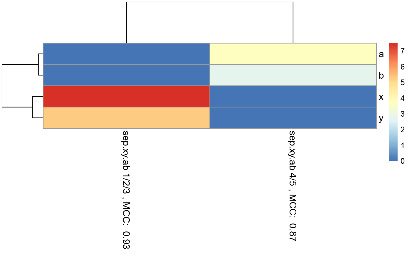
#Make example data where samples with 1, 2, and 3 in their ID names can be
#predicted using features x and y, while samples with 4 and 5 in their ID names
#can be predicted using features a and b.

id = c("1a", "1b", "1c", "1d", "1e", "1f", "1g", "2a", "2b", "2c", "2d", "2e", "2f", "3a",
       "3b", "3c", "3d", "3e", "3f", "3g", "3h", "3i",
       "4a", "4b", "4c", "4d", "4e", "4f", "4g", "5a", "5b", "5c",
       "5d", "5e", "5f", "5g")

x = c(18, 21, 22, 24, 26, 26, 27, 30, 31, 35, 39, 35, 30, 40, 41, 42, 44, 46, 47, 48, 49, 54,
1, 1, 1, 1, 1, 1, 1, 1, 1, 1, 1, 1, 1, 1)

y = c(10, 11, 22, 15, 12, 13, 14, 33, 39, 37, 44, 40, 45, 27, 29, 20, 28, 21, 30, 31, 23, 24,
1, 1, 1, 1, 1, 1, 1, 1, 1, 1, 1, 1, 1, 1)

a = c(1, 1, 1, 1, 1, 1, 1, 1, 1, 1, 1, 1, 1, 1, 1, 1, 1, 1, 1, 1, 1, 1,
18, 21, 22, 24, 26, 26, 27, 40, 41, 42, 44, 46, 47, 48)

b = c(1, 1, 1, 1, 1, 1, 1, 1, 1, 1, 1, 1, 1, 1, 1, 1, 1, 1, 1, 1, 1, 1,
10, 11, 22, 15, 12, 13, 14, 27, 29, 20, 28, 21, 30, 31)

sep.xy.ab = c("1/2/3", "1/2/3", "1/2/3", "1/2/3", "1/2/3", "1/2/3", "1/2/3",
"1/2/3", "1/2/3", "1/2/3", "1/2/3", "1/2/3", "1/2/3", "1/2/3", "1/2/3", "1/2/3",
"1/2/3", "1/2/3", "1/2/3", "1/2/3", "1/2/3", "1/2/3",
"4/5", "4/5", "4/5", "4/5", "4/5", "4/5", "4/5", "4/5", "4/5", "4/5", "4/5",
"4/5", "4/5", "4/5")

actual = as.factor(c("1", "1", "1", "1", "1", "1", "1", "2", "2", "2", "2", "2", "2", "3", "3", "3",
       "3", "3", "3", "3", "3", "3", "4", "4", "4", "4", "4", "4", "4", "5", "5", "5", "5", "5",
       "5", "5"))

example.data <- data.frame(id, x, y, a, b, sep.xy.ab, actual)

#dev.new()
plot(example.data$x, example.data$y)
text(example.data$x, example.data$y,labels=example.data$id)

#dev.new()
plot(example.data$a, example.data$b)
text(example.data$a, example.data$b,labels=example.data$id)

results <- RandomForestClassificationGiniMatrixForPheatmap(input.data = example.data,
                                       factor.name.for.subsetting = "sep.xy.ab",
                                       name.of.predictors.to.use = c("x", "y", "a", "b"),
                                       target.column.name = "actual",
                                       seed = 2)

matrix.for.pheatmap <- results[[1]]

#Add MCC to column names
for(i in 1:dim(matrix.for.pheatmap)[2])
{
   old.name <- colnames(matrix.for.pheatmap)[[i]]
   MCC.val <- matrix.for.pheatmap[dim(matrix.for.pheatmap)[1],][[i]]
   new.name <- paste(old.name, ", MCC: ", format(round(MCC.val, 2), nsmall = 2))
   colnames(matrix.for.pheatmap)[[i]] <- new.name
}

#Remove MCC row from matrix
matrix.for.pheatmap.MCC.row.removed <- matrix.for.pheatmap[1:(dim(matrix.for.pheatmap)[1]-1),]

pheatmap_RF <- pheatmap::pheatmap(matrix.for.pheatmap.MCC.row.removed, fontsize_col = 12,
fontsize_row=12)


#The pheatmap shows that the points in groups 1, 2, and 3 can be predicted
#with features x and y. While points in group 4 and 5 can be predicted with
#features a and b.
#dev.new()
pheatmap_RF

#Note that the 1/2/3 column is exactly the same as the random forest
#model created in the example for eval.classification.results.
#Since this pheatmap is using the number of LOOCV rounds
#as the input matrix, the colors can be misleading. It looks
#like features x and y are more important for 1/2/3 than features a and b
#is for 4/5. However, this is not the case. The mean decrease
#in gini index cannot be used to compare features between models. It
#can only be used to compare features within a single model.

Arguments

Value

Details

See also

Examples